R Squared: Difference between revisions
| (17 intermediate revisions by the same user not shown) | |||
| Line 1: | Line 1: | ||
=Introduction= | =Introduction= | ||
This is all about R² and | This is all about R². | ||
=My Thoughts= | |||
==Least Squares Review== | |||
Most of this requires you to think about a dataset with lots of points. What we are trying to do is with [[least squares | least squares]] is find the best fit for a line for our data points. Once we have this we could maybe predict for a new data point what the y-value might be given the x-value. Here is the formula | |||
<br> | |||
<math> | |||
S = \sum_{i=1}^n (y_i - \hat{y}_i)^2 | |||
</math> | |||
<br> | |||
And here is an example of usage<br> | |||
[[File:Lsq9.png|600px]]<br> | |||
==R Squared== | |||
With <math>R^2</math> we are looking at the variances (changes) using the mean and the line. Squaring means we don't care about negative or positive. | |||
=What is the difference= | =What is the difference= | ||
Well I guess R² = R squared. R² is the variance between a dependent variable and an independent variable in terms of percentage. Therefore 0.4 R² = 40% and R = 0.2. I guess I agree that using R² does provide an easier way to understand what you mean however there is no sign on R². | Well I guess R² = R squared. R² is the variance between a dependent variable and an independent variable in terms of percentage. Therefore 0.4 R² = 40% and R = 0.2. I guess I agree that using R² does provide an easier way to understand what you mean however there is no sign on R². | ||
| Line 6: | Line 19: | ||
This is given by<br> | This is given by<br> | ||
[[File:Rsquared.png|400px]]<br> | [[File:Rsquared.png|400px]]<br> | ||
A reminder of how we calculate variance, we add up the differences from the mean like below. '''Note''' this shows a population and we should divide by n-1 not n but I liked the graphic.<br> | |||
[[File:Pop var.png|600px]]<br> | [[File:Pop var.png|600px]]<br> | ||
This was a nice picture<br> | |||
[[File:Variance cal.png|400px]] | |||
=F= | |||
Spent a lot of time looking a this but got nowhere. It is a way to get a p-value. For F the following formula we given.<br> | |||
[[File:F formula.png| 200px]]<br> | |||
The Pfit and Pmean explanations were provided. Pfit was the number of parameters. E.g. for mouse we could look at weight, size and tail. And the Pmean was the number of means, which is normally 1. The n is the number not explained by the fit. This took a while but I believe this to be the residuals Observed (y) - Predicted (y_hat). | |||
[[File:R2 Summary.png]] | |||
Latest revision as of 03:49, 23 April 2025
Introduction
This is all about R².
My Thoughts
Least Squares Review
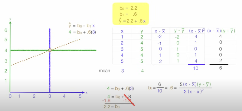
Most of this requires you to think about a dataset with lots of points. What we are trying to do is with least squares is find the best fit for a line for our data points. Once we have this we could maybe predict for a new data point what the y-value might be given the x-value. Here is the formula
And here is an example of usage

R Squared
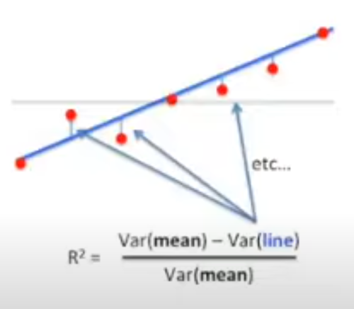
With we are looking at the variances (changes) using the mean and the line. Squaring means we don't care about negative or positive.
What is the difference
Well I guess R² = R squared. R² is the variance between a dependent variable and an independent variable in terms of percentage. Therefore 0.4 R² = 40% and R = 0.2. I guess I agree that using R² does provide an easier way to understand what you mean however there is no sign on R².
Formula for R²
This is given by

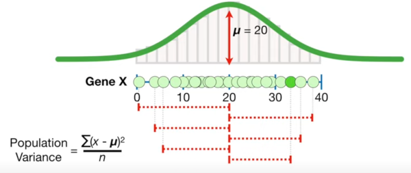
A reminder of how we calculate variance, we add up the differences from the mean like below. Note this shows a population and we should divide by n-1 not n but I liked the graphic.

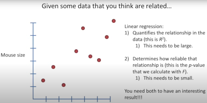
This was a nice picture

F
Spent a lot of time looking a this but got nowhere. It is a way to get a p-value. For F the following formula we given.
![]()
The Pfit and Pmean explanations were provided. Pfit was the number of parameters. E.g. for mouse we could look at weight, size and tail. And the Pmean was the number of means, which is normally 1. The n is the number not explained by the fit. This took a while but I believe this to be the residuals Observed (y) - Predicted (y_hat).
