Matrices and Vectors

Introduction

Next as the title says

Example

Here we go

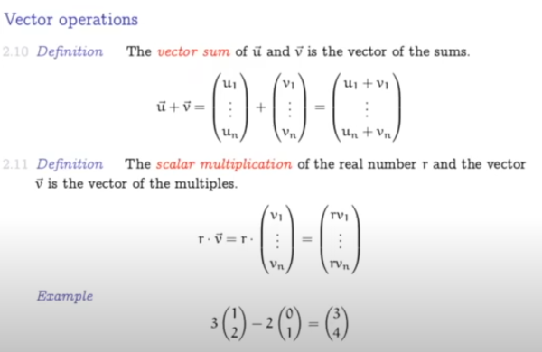
Vector Operations

We can add the components or scale them provided they are the same size

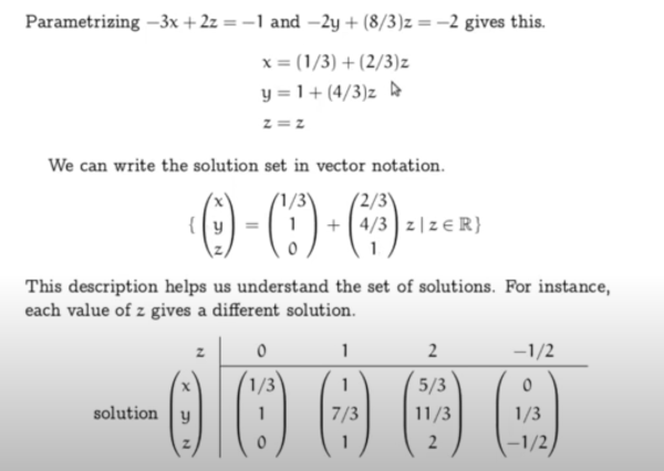
Gaussian as Vectors

And here are the linear equations using gaussian and vectors

Homegenous Systems

Homegenous Systems always has a least one solution. Watching an alternative video showed the questions using the form 2x₁ + 4x₂ rather than 2a + 4b. There are two types of Homegenous Systems, trivial and non-trivial. The trivial solution is where all the variables are = to zero. This demonstration helped a lot in how to solve this. Here was the question

$\begin{array}{r}1x_1+2x_2+3x_3+2x_4=0\\ 1x_1+3x_2+5x_3+5x_4=0\\ 2x_1+4x_2+7x_3+1x_4=0\\ -1x_1-2x_2-6x_3+7x_4=0\end{array}$
Putting it into augmented matrices

\begin{bmatrix} 1 & 2 & 3 & 2 & | & 0 \\ 1 & 3 & 5 & 5 & | & 0 \\ 2 & 4 & 7 & 1 & | & 0 \\ -1 & -2 & -6 & 7 & | & 0 \end{bmatrix}

$\begin{array}{r}-1R_1+R_2\to R_2\\ -2R_1+R_3\to R_3\\ R_1+R_4\to R_4\end{array}$

\begin{bmatrix} 1 & 2 & 3 & 2 & | & 0 \\ 0 & 1 & 2 & 3 & | & 0 \\ 0 & 0 & 1 & -3 & | & 0 \\ 0 & 0 & -3 & 9 & | & 0 \end{bmatrix}

$\frac{1}{3}{R}_4\to R_4$

\begin{bmatrix} 1 & 2 & 3 & 2 & | & 0 \\ 0 & 1 & 2 & 3 & | & 0 \\ 0 & 0 & 1 & -3 & | & 0 \\ 0 & 0 & -1 & 3 & | & 0 \end{bmatrix} Next we do the following

$\begin{array}{r}{R}_3+R_1\to R_1\\ -2R_3+R_2\to R_2\\ -1R_3+R_4\to R_4\end{array}$

\begin{bmatrix} 1 & 0 & 0 & -7 & | & 0 \\ 0 & 1 & 0 & 9 & | & 0 \\ 0 & 0 & 1 & -3 & | & 0 \\ 0 & 0 & 0 & 0 & | & 0 \end{bmatrix} Putting back variables and losing the 0 line
$\begin{array}{r}1x_1+7x_4=0\\ 1x_2+9x_4=0\\ 1x_3-3x_4=0\end{array}$
We can now express $x_4$ and derive the other variable in terms of k $\begin{array}{r}{x}_3=3k\\ x_2=9k\\ x_1=7k\end{array}$

This means list the solution in terms of x, i.e. x₁,x₂,x₃,x₄ gives

(7k, 9k, 3k, k)

So taking k = 1 would be

(7, 9, 3, 1)

You can put this in the original problem and it works

Terms

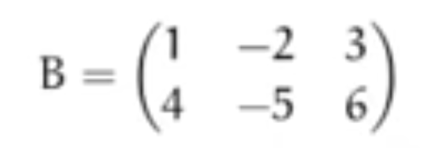
• m x n a matrix of m row, n colums
• Capital let for name of Matrix
• Small letter for entry
• nonsingular is a unique homegeneous solution
• singular is a homegeneous with infinite solutions