Machine Learning Course

Introduction

This is to capture some terms in machine learning course

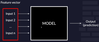
Terms

They discussed the following

Types of Learning

• Supervised
• Unsupervised
• Reinforcement Learning

Supervised Learning :This type uses labeled data, where the input and desired output are known, to train a model. The model learns to map inputs to outputs, allowing it to make predictions on new, unseen data. Examples include:

• Classification: Predicting categories (e.g., identifying spam emails).
• Regression: Predicting continuous values (e.g., predicting house prices).
  

Unsupervised Learning :This type works with unlabeled data, where there are no predefined outputs or target variables. The model's goal is to discover patterns, relationships, or structures within the data. Examples include:

• Clustering: Grouping similar data points together (e.g., customer segmentation).
• Dimensionality Reduction: Simplifying data by reducing the number of variables while preserving important information.
  

Reinforcement Learning :This type involves training an agent to learn how to make decisions in an environment to maximize a reward signal. The agent learns through trial and error, receiving rewards or penalties for its actions. Examples include:

• Game Playing: Training an AI to play games like Go or chess.
• Robotics: Controlling robots to perform tasks effectively.

Types of Data

• Nominal data
• Ordinal data
• Discrete data
• Continuous data

Nominal Attributes : Nominal attributes, as related to names, refer to categorical data where the values represent different categories or labels without any inherent order or ranking. These attributes are often used to represent names or labels associated with objects, entities, or concepts. Example colours, Sex

Ordinal Attributes : Ordinal attributes are a type of qualitative attribute where the values possess a meaningful order or ranking, but the magnitude between values is not precisely quantified. In other words, while the order of values indicates their relative importance or precedence, the numerical difference between them is not standardized or known. Example grades, payscale

Discrete : Discrete data refer to information that can take on specific, separate values rather than a continuous range. These values are often distinct and separate from one another, and they can be either numerical or categorical in nature. Example Profession, Zip Code

Continuous : Continuous data, unlike discrete data, can take on an infinite number of possible values within a given range. It is characterized by being able to assume any value within a specified interval, often including fractional or decimal values. Example Height, Weight

Datasets for Supervised Learning

• Validation Dataset
• Training Dataset
• Test Dataset

Training Dataset: This dataset is used to train the supervised learning model. It contains labeled examples of both inputs (features) and corresponding outputs (labels).

Validation Dataset: This dataset is a subset of the training data that is held out during training and used to evaluate the model's performance. It helps to identify overfitting, which is when the model learns the training data too well and performs poorly on unseen data.

Test Dataset: This dataset is completely separate from the training and validation datasets and is used for a final, independent evaluation of the model's generalization ability. The test dataset should be used only after the model has been trained and validated to get a true measure of how well the model will perform in real-world scenarios.

Loss explained

Loos is the comparison between the model output and the actual result. The smaller the number the better the model.

How they Processed the data

Changed the classification

In the data there were two categories of data, g and h. This was changed a number e.g. g=0, h=0

Put the data into a histgoram

This just aloud you to visualize the data

Oversampled

When they looked a the data there were more of one category than the other. Rather than remove data they used the lesser dataset to make more of the data to equal the other. This was only done for training set

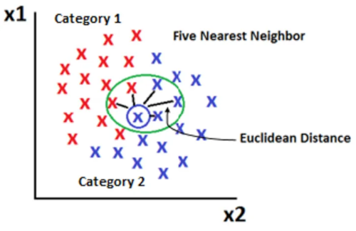
K Nearest Neighbour

They calculated the nearest neighbour. This is where you measure the distance between a new point and the neighbours. I think I have done this before

The important outputs for this were Precision, Recall and F1 Score
Relevant Instances : Relevant Instances are the actual correct examples in the dataset that the model is trying to identify. Also known as Ground Truth
Retrieved Instances : Retrieved Instances are the number of images in the dataset relevant to the query. E.g. if you have 3 classifications , the Retrieved Instances will be the count of the items which are that classification

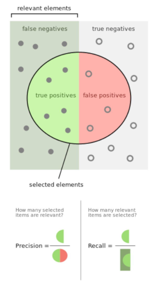
Precision (how many predicted positives are correct)
Suppose you are classifying images of bears into three categories: "grizzly," "black," and "teddy." If your model predicts 50 images as "grizzly," but only 45 of them are actually "grizzly" (and 5 are not), the precision for the "grizzly" class would be:

Precision = 45 / (45 + 5) = 0.9 (or 90%)

Recall (how many actual positives are identified)
Suppose you are classifying images of bears into three categories: "grizzly," "black," and "teddy." If there are 100 images of "grizzly" bears, and your model correctly identifies 90 of them as "grizzly" but misses 10 (classifies them as another type), the recall for the "grizzly" class would be:

Recall = 90 / (90 + 10) = 0.9 (or 90%)

There are difference formulas for calculating the distance

• Euclidean
• Manhattan or
• Hamming

They used Euclidean

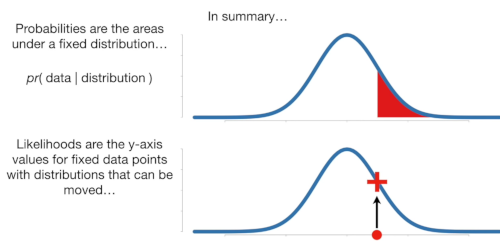
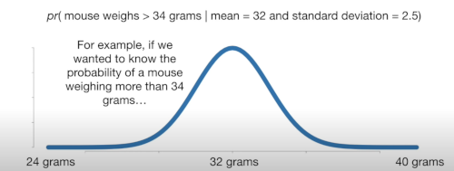
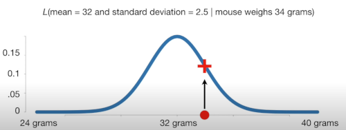
Difference between Probability and Likelyhood

So this was enlightening

Probability

Likelyhood

Conditional Probability

Long time since I did this so here is a refresher for me. So here is a big picture to remind me about probability first (which I do know)

Conditional probability is the likelihood of an event or outcome occurring, based on the occurrence of a previous event or outcome. The formula for this is

The bar | refers to given and means B has occurred. The upside u (∩) is the intersection. So where A intersects B. Lets get a venn diagram to demonstrate

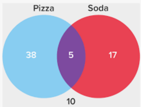
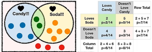
We can document the probabilities in a 'contingency table

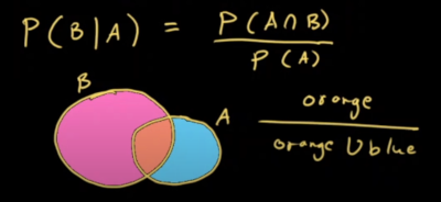
I liked this picture to demonstrate the formula. Orange / Orange ∪ Blue. Where ∪ is union or two sets

The Chain Rule (Probability)

This is a rule which shows you how to find the probability when you want to consider the other events. Turns out there are two of these. We want probability. And we are back on to intersections and events. We are looking for an answer to this

P(A₁ ∩ A₂ ∩ ... ∩ Aₙ) 

So we can express this for four events in the chain rule like this

P(A₁ ∩ A₂ ∩ A₃ n A₄) = 
   P(A₁) . 
   P(A₂ | A₁) . 
   P(A₃ | A₁ ∩ A₂) .
   P(A₄ | A₁ ∩ A₂ ∩ A₃)

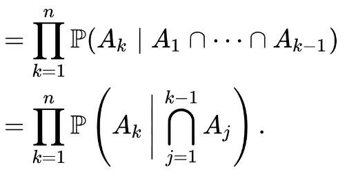
Or to put it another fancier way we can use the Capital Pi

Naive Bayes

Introduction

So I struggled a lot with this because I thought it was complicated but it isn't. It is really simple. Basically it is this formula.

P(A|B) = ( P(B|A) * P(A) ) / P(B)

Given A What is the probability of A occurring given B. What complicated it for me was not putting in those terms. I originally thought there were two formulas as I have watched two video which seemed vastly different.

Throughout they used a football analogy where the classification was whether you would play football or not i.e. yes or no. This would be based on different events like, day of the week, weather, sex, etc. The key thing with Bayes was the these events are independent of each other. In the [chain rule] we consider probabilities in context to the other events, e.g. Of the day of the week, and the males, and it being sunny whats the probability of you playing. With Bayes we consider one thing independently of the others.
Usually using the validation data we find the probability of whether we played (the classification), e.g. out of 100, 25 played, so that would be .25. Then you use Bayes to calculate the individual events using Bayes. So what is the probability of

male given the probability of playing football
sunny  given the probability of playing football
monday  given the probability of playing football

We multiply them out and see which is the biggest and that is it.
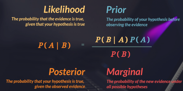
So I guess I need to document the terms for this. I did watch this video which was guess good. Now some terms and a pretty picture

• Likelihood
• Prior
• Posterior
• Marginal

Bayes Theorem (Same Thing)

This is from the video. I was using to make this page
Because I did not understand I ended up googling Bayes and found they referred to it as Bayes Theorem but it is the same thing
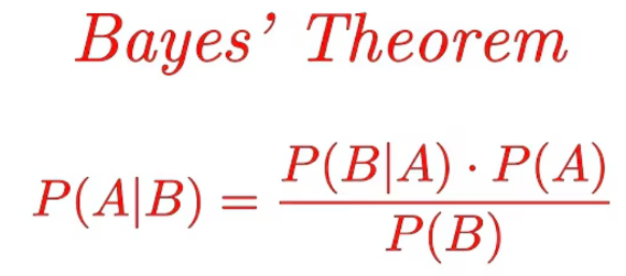
Where

• P(A|B): The probability of event A occurring given that event B has occurred (posterior probability).
• P(B|A): The probability of event B occurring given that event A has occurred (likelihood).
• P(A): The probability of event A occurring (prior probability).
• P(B): The probability of event B occurring (evidence or marginal probability).

To me it was also helpful to see the venn diagram. If we look at the Conditional Probability again reorganized the original formula

P(A ∩ B ) = P(A|B) * P(B)

We can see that that if we take the denominator to Bayes to the left side we have

P(A|B) * P(B) = P(B|A) * P(A)  

Worked Example From Stats Quest Style

This is not to be confused with Gaussian Naive Bayes below. This is a lot easier on the brain. You take a histogram of the categories you care about. In this case words for both spam and normal messages and calculate the probability separately for each.

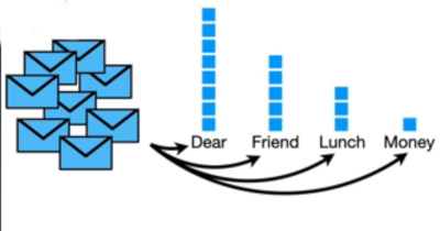
Now you have probabilities for each case

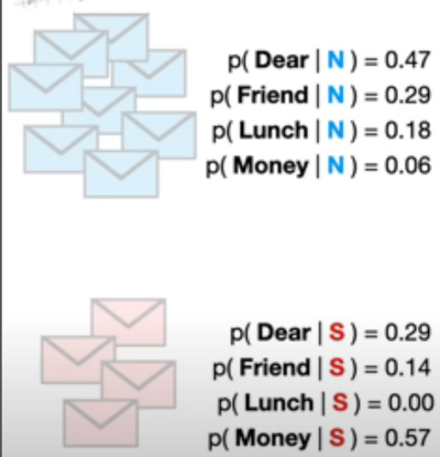
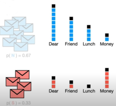
We then create an initial guess on for each on whether this is a normal message. In the video they used the classified dataset to do this but were keen to stress guess. For their set there were 12 messages and 8 were ok
For normal

0.67

For spam

0.33 

Next they looked at a scenario where an emailed contained Dear and Friend. So To do this we use

p(initial Guess | Dear Friend)

For normal message

p(.067 x 0.47 x 0.29) = 0.09

For spam

p(0.33 x 0.29 x 0.14 = 0.01

So a email with Dear Friend in it is a normal message as 0.09 > 0.01
You may notice that the average for Lunch for spam is 0. This causes problems as all the results with Lunch will be zero. To work around this they add a number of counts to each category. This is referred to as a (alpha)

Second Example

So here is the example from the video. I was looking it to be harder than it was.

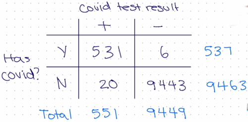
I think the problem was that it didn't look like the previous examples but it is, Has Covid (y/n) is the classification and positive/negative is the event Not sure if the numbers match but we were given

P(false +Test) = 0.05
P(false -Test) = 0.01
P(having decease) = 0.1

What is the probablity of

P(having decease|+ test)

The person drew a diagram

               +     -
            ------------
Has Covid         | 0.01
No  Covid   0.05  |

Given the rows must equal 100 as they are percentages we now have

               +     -
            ------------
Has Covid   0.99  | 0.01
No  Covid   0.05  | 0.95

Using the formula above

P(A|B) = (P(B|A) * P(A)) / P(B)
P(+Test | Has Covid) = P(Has Covid|+Test )*P(Has Covid) / P(+Test)
0.1 * 0.99 / P(+Test)

Given the lack of context when I watched this, I could not understand what they were saying so calculating P(+Test) was hard to grasp. Now I know I feel a fool. Basically we want to calculate the probability of getting a +Test for each classification (has Covid/No Covid). So what is the probability I have a positive test

• and I do have the decease 0.99 +Test given 0.1 has covid
• and do not have the decease 0.05 +Test given 0.9 has covid

This now works out to be

= 0.99 * 0.1 / ((0.99 * 0.1) + (0.05 * 0.9))
= .6875 = 68.75%

The Formula

Introduction

So this now leads me to this wonderful piece of formula

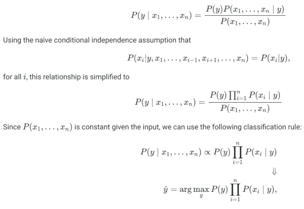
I think the second line is maybe a mistake or extra information as I could not track this down.

Capitol Pi (Π)

This is used in the formula, so here is an explanation of Capital Pi. It is similar to Sigma but with capital Pi you multiply inside of add.

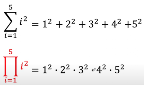
Formula Explanation

So the first bit is just Bayes theorem with for each feature.

P(y|x) = (P(y) * P(x|y) ) / P(x)

Which in english is

posterior =  (prior x likelihood) / evidence

It most of the documents I have seen Cₖ to denote Classification k. So the left hand side of the formula can we express in english by saying what is the probability of we are in classification k given these inputs. E.g. Should I play football today (the Classification yes/no) given it's raining, and wind and weekend.... (inputs x₁...xₙ).

Using the chain rule we can express this as

P(Cₖ|x₁...xₙ) 
  = P(x₁...xₙ,Cₖ)
  = P(x₁|x₂...xₙ,Cₖ) . P(x₂...xₙ,Cₖ)
  = P(x₁|x₂...xₙ,Cₖ) . P(x₂|x₃...xₙ,Cₖ) . P(x₃...xₙ,Cₖ).
  = P(x₁|x₂...xₙ,Cₖ) . P(x₂|x₃...xₙ,Cₖ) . P(x₃...xₙ,Cₖ) ...
      P(xₙ₋1 | xₙ, Cₖ) . P(xₙ | Cₖ) . P(Cₖ)

Now we come on to conditional independence. This proposes the events we are observing are independent of each other. Testing to see if we play soccer, rain and day of week, or other features are all independent (big assumption and what puts the naive in Bayes). This bit took a while to sink in. Because of our assumption these are independent we do not need to chain the values together like the example above, instead we do calculate the probability for just to that that instance of i

P(xᵢ|xᵢ₊₁...xₙ,Cₖ) = P(xᵢ | Cₖ)

Now the rule for Naive Bayes where ∝ means proportional Next bit took a while. The P(xᵢ₊₁...xₙ) is the same for each event. If we took three numbers, 10,20,30 and divided them by the same value it would not change the which was the biggest e.g.

10/2, 20/2, 30/2 
10/4, 20/4, 30/4 

The order smallest to largest is always the same. For Bayes this is what we care about, which is the biggest number, not the number itself. Finally we get to the last line. The y is in our case k. So we calculate the probabilities for each event for each Classifier and we take the biggest one.
The predicted value is called y-hat or ŷ and is used to denote a predicted value rather than an actual value.

Logistic Regression

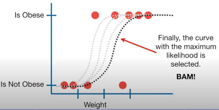
This approach uses a decision boundary to separate classifications. This is typically represented by a sigmoid curve

$P(y=1)=\frac{1}{1+e^{-({\beta }_0+{\beta }_{1}x)}}$

Here is an example of testing if the weight of a mouse determines if a mouse is obese.